Churn Prediction - Comparing Multiple Models

Abstract

This project report delves into identifying critical factors and the most effective predictive model for customer churn at a Dutch energy provider, a pressing issue in the competitive European energy sector. By meticulously analyzing a dataset of 20,000 customer observations, the study executed a thorough data preparation process including outlier removal and the introduction of a new variable for better understanding customer behavior. The investigation compared various predictive models, including Logistic Regression, Decision Trees, Gradient Boosting, and others, concluding that Gradient Boosting outperformed the rest. Key findings underscore the significance of service usage, relationship length, contract length, and flexible contracts in influencing customer churn. Notably, longer relationships and contract durations correlated with lower churn rates. The report suggests that the energy supplier could enhance customer retention strategies by focusing on long-term relationships and stable contract terms, alongside developing energy efficiency programs for high-usage customers, thereby fostering loyalty and reducing churn.

Managerial Summary

This project is dedicated to identifying the key factors and the most effective model for predicting customer churn for a Dutch energy provider. This task is especially critical in the European energy sector, where market liberalization has ramped up competition, making customer retention maybe the most important focus for companies in this sector.

The examined dataset consists of 20,000 customer observations, carefully refined through a comprehensive data cleaning and preparation process. This involved the identification and removal of outliers, particularly in critical variables such as income, electricity, and gas usage, to enhance the integrity of the analysis. Additionally, a new variable is introduced to better understand customer behavior, the “flexible_contract”, on which contracts could be terminated at any time.
The baseline model for this study comprises a logistic regression model and it is constructed based on the study’s hypotheses, deriving from the literature review and the exploratory analysis. As a result, it includes the variables gender, age, income, relation length, electricity usage, gas usage, contract length, and flexible contract. Subsequently, different methods are implemented to test their performance and to determine the most important attributes for the specific task. The methods under comparison are Logistic Regression, Stepwise Logistic Regression, Decision Tree model, Gradient Boosting, Random Forest, Support Vector Machine, and Neural Network. The model that emerged as the better performing based on various evaluation metrics is the gradient boosting model.

Regarding the most important attributes, this study highlights several key variables significantly impacting customer churn. Service usage, relationship length, and contract length are the most influential determinants. Notably, customers with longer relationships and more extended contract terms exhibited lower churn rates.

In conclusion, the energy supplier can tailor their customer retention strategies more effectively, focusing on long-term relationships, and stable contract terms, and develop energy efficiency programs for customers with higher energy usage.

Data Description

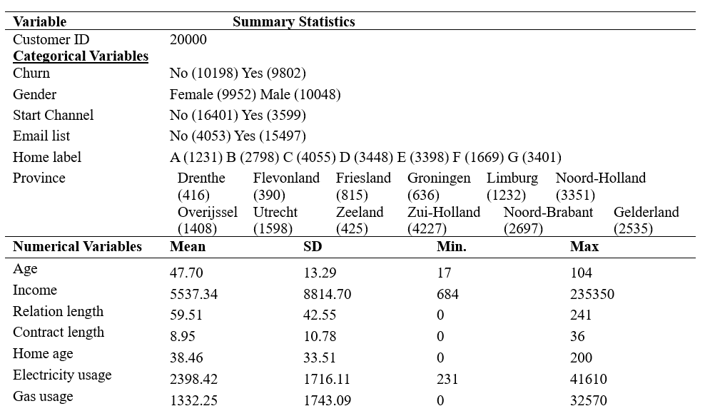
The dataset, comprising 20,000 customer observations from a Dutch energy supplier, underwent an initial summary check to identify any potential anomalies. The examination revealed the absence of any missing values within the dataset. The variables are converted to different types, in order to give them the appropriate format. A descriptive statistics table for numerical and categorical variables is then created (Table 1). Based on this table, important insights are gained. It is noticed that most of the customers are older and have moderate income. Most of the customers are loyal as the mean relationship length is almost 5 years.

*For a detailed description of the different factors, refer to Appendix 1

Data Descriptives

Data Cleaning & EDA

The first step in the EDA and data cleaning process involves checking for missing values, while the second step focuses on converting factors into their appropriate forms

# Data Cleaning & Descriptives ----
# Reviewing missing values 
for(col in names(data)) { 
  missing_values <- sum(is.na(data[[col]]))
  print(paste("Column", col, "has", missing_values, "missing values."))}
# no missings
# Removing Customer_ID
data$Customer_ID <- NULL
# Convert the variables into the appropriate form
# columns to convert
factor_var <- c('Churn', 'Gender', 'Email_list', 'Home_label', 'Start_channel', 'Province')
numeric_var <- c('Electricity_usage', 'Gas_usage', 'Income')
integer_var <- c('Age', 'Home_age', 'Relation_length', 'Contract_length')
# Converting factor variables
for(var in factor_var){
  data[[var]] <- as.factor(data[[var]])}
# Converting numeric variables
for(var in numeric_var){
  data[[var]] <- as.numeric(data[[var]])}
# Converting integer variables
for(var in integer_var){
  data[[var]] <- as.integer(data[[var]])}

The data exploration process indicated the absence of missing values within the dataset. The subsequent step entails examining the distribution of numerical variables to identify any potential outliers.

# Convert data from wide to long format using pivot_longer
long_data <- data %>%
  pivot_longer(cols = c(Electricity_usage, Gas_usage, Income), names_to = "Variable", values_to = "Value")

# Plot with ggplot2
ggplot(long_data, aes(x = Variable, y = Value)) +
  geom_boxplot() +
  facet_wrap(~ Variable, scales = "free_x", nrow = 1) +
  labs(x = NULL, y = "Value") +
  theme_minimal() +
  theme(axis.text.x = element_text(angle = 45, hjust = 1))

Outliers in variables, “Income,” “Electricity_usage,” and “Gas_usage” were identified through the use of boxplots. This method highlights data points that lie outside the expected range. Further statistical analysis of summary statistics, has indicated significant deviations in these variables, especially in terms of their mean and standard deviations. This was evident in the case of “Income,” where values ranged at 235,350, with a mean of approximately 5,537 and a substantial standard deviation, indicating a widespread. Similarly, “Electricity_usage” showed a maximum value of 41,610, exceeding the mean usage of about 2,398, and “Gas_usage” peaked at 32,570, which was much higher than its mean of 1,332. These deviations highlight the presence of outliers that could potentially affect the overall analysis. Thus, it is considered that extremely high values in “Income”, Electricity_usage” and “Gas_usage,” may not accurately represent the general customer base, indicating anomalies, measurement errors, or data entry errors. Driven by the necessity to maintain data quality, ensuring that the analysis reflects the typical customer profile and is not skewed by extreme, atypical values, we proceed to the removal of these outliers. The methodology for the removal of these outliers is described below. By plotting the boxplots, it is observed that income, electricity, and gas usage have significant outliers and based on their values they were deleted. The number of observations is diminished to 19699. Below, it is explained analytically.

Income: All variables above value 30042 were deleted, as it was determined that this is the point where the values experience a significant breakpoint. This was done by calculating the point at which the greatest difference between the values of the variable is noticed. With only 60 variables (0.3%) having an income value above 30042, it was determined that deleting them wouldn’t skew the data negatively, due to the insignificant amount. Deletion was chosen over completion to minimize noise, simplify and strengthen the models, and avoid overfitting.

Electricity Usage: All variables above 9000 in electricity usage were deleted. This was discovered through plot analysis and studying the units at the change points, with sorting employed for easier and clearer understanding. Given that only 117 variables (0.585%) had electricity usage above 9000, it was determined that their deletion wouldn’t negatively skew the data, due to the insignificant amount.

Gas Usage: All variables above 3209 were deleted using the same method as with the income. With only 125 variables (0.625%) having electricity usage above 3209, it was determined that deleting them wouldn’t negatively skew the data, given the insignificant amount.

Age: It was chosen to remove all values where the age is less than 18, as it logically doesn’t make sense for someone who is not an adult to have a contract with the company

Correlation Matrix

# Exploratory Analysis -----
## How many customers have churned
# Corelation Matrix
data_numeric <- data %>%
  mutate_if(is.factor, as.integer) %>%
  mutate_if(is.character, function(x) as.integer(factor(x))) 
cor_matrix <- cor(data_numeric, use = "complete.obs")
melted_cor_matrix <- melt(cor_matrix)
unique_vars <- unique(c(melted_cor_matrix$Var1, melted_cor_matrix$Var2))
var_mapping <- setNames(seq_along(unique_vars), unique_vars)
melted_cor_matrix$Var1 <- var_mapping[as.character(melted_cor_matrix$Var1)]
melted_cor_matrix$Var2 <- var_mapping[as.character(melted_cor_matrix$Var2)]
melted_cor_matrix <- melted_cor_matrix %>%
  filter(Var1 <= Var2)  # Include the diagonal
# Create the Correlation heatmap Matrix
ggplot(melted_cor_matrix, aes(x = Var1, y = Var2, fill = value)) +
  geom_tile() +
  geom_text(aes(label = sprintf("%.2f", value)), color = "black", size = 3, check_overlap = TRUE) +
  scale_fill_gradient2(low = "blue", high = "red", mid = "white", midpoint = 0, limit = c(-1, 1)) +
  scale_x_continuous(breaks = var_mapping, labels = names(var_mapping)) +
  scale_y_continuous(breaks = var_mapping, labels = names(var_mapping)) +
  theme_minimal() +
  labs(title = "Correlation Matrix Heatmap (Lower Triangle)", x = "", y = "") +
  theme(axis.text.x = element_text(angle = 45, vjust = 1, hjust = 1))

The variables with the strongest negative correlations are age, relationship length, contract length, flexible contract (the strongest), and start channel, indicating that churn decreases as these variables increase. Conversely, home age, electricity, and gas use show the strongest positive correlations, meaning churn increases as these variables increase. These being the variables with the strongest statistical influence on churn, their relationship was studied more closely. The relationships of each variable with churn are then examined using plots and appropriate tests (chi-squared test and logit regression), revealing significant associations with churn for all variables.

Dependent - Independent Variables Relationship

## Discrete Variables 
## Relation length (Significant)
ggplot(data, aes(x = Relation_length, y = Churn, fill = Churn)) + 
  stat_summary(fun = "mean", geom = "col") +
  labs(title = "Mean Relation Length of Remaining vs Churned Customers") +
  theme_bw()

## Start_channel (Significant) 
ggplot(data, aes(x = Start_channel, fill = Churn)) +
  geom_bar(position = "dodge") +
  labs(x="Start Channel", y="Churn Amount", title="Churn per Start Channel") +
  scale_fill_manual(values=c("#FF4136", "#2ECC40"), labels=c("No", "Yes")) +
  theme_bw()

## Electricity usage (Significant)
ggplot(data, aes(x = Electricity_usage, y = Churn, fill = Churn)) + 
  stat_summary(fun = "mean", geom = "col") +
  labs(title = "Mean Electricity Usage of Remaining vs Churned Customers") +
  theme_bw()

The analysis of customer behavior reveals that a significant portion of high electricity and gas usage customers have experienced churn. Notably, customers with flexible contracts, indicative of shorter relationship lengths, show a higher likelihood of churning. Furthermore, the acquisition channels play a role in customer retention. The company has acquired a greater number of customers online compared to phone acquisitions. Interestingly, a higher percentage of customers acquired online have churned, while a larger proportion of customers acquired through phone interactions have remained loyal to the company.

Model Estimation and Evaluation

The baseline model in this study is a logistic regression model, developed from the hypotheses generated through literature review and exploratory analysis. This model incorporates variables such as gender, age, income, relationship duration, electricity and gas consumption, contract length, and the availability of a flexible contract. To evaluate their efficacy and identify the key factors for this specific task, various methods are tested, including Logistic Regression, Stepwise Logistic Regression, Decision Tree model, Gradient Boosting, Random Forest, Support Vector Machine, and Neural Network.

To determine the best-performing model, various metrics are employed. The body of literature on churn management encompasses a wide range of metrics for evaluating the effectiveness of models designed for predicting customer churn. The Hit ratio helps to measure the model’s accuracy and tries to correctly identify the positive cases of a logistic regression. One limitation is that it doesn’t identify the false positives of the model. The Top Decile Lift tells us how effective the model is in ranking predictions. It does that by splitting the predictions into deciles (10 groups of the same size) and comparing the 10th decile with a random selection or with another model. The Area Under the Curve (AUC) is a metric used to evaluate the performance of a binary classification model, it measures the ability of the model to distinguish between positive and negative examples. Finally, the Gini coefficient aids in studying the distribution in model evaluation and is particularly helpful when deciding between two classes.

Logistic Regression

Logit models are a class of models used to explore the relationship of a dichotomous dependent variable to one or more independent variables. (Gottman, J., & Roy, A., 1990). The logit model estimates the probability that an event will happen or not (in our case, it predicts if the customer will churn). In action, it shows to which extent the independent variables will influence the event (churn) and in what way.

The baseline model for this study is constructed based on the study’s hypotheses deriving from the literature review and the exploratory analysis. As a result, the baseline model consists of the variables gender, age, income, relation length, electricity usage, gas usage, contract length, and flexible contract. However, because contract length and flexible contract are highly correlated and the inclusion of both possibly causes multicollinearity problems, the flexible contract is selected since it has a greater negative correlation with the dependent variable.

The dataset is split into a training set (75%) and a testing set (25%). The former is used for the estimation and training of the model while the latter is for the evaluation of its performance when a new dataset is introduced. The estimation of the baseline model presents that most of the baseline variables are statistically significant for predicting churn, except for gender and age. This finding suggests evidence that the initial hypothesis which states that males have a greater probability to churn is rejected, similar to the hypothesis that age younger individuals have a greater possibility of defecting.

# Logistic Regression 
#Get a 75% estimation sample and 25% validation sample
set.seed(1234)
data$estimation_dataset <-rbinom(nrow(data), 1, 0.75)
estimation_dataset <- data[data$estimation_dataset == 1,]
validation_dataset<- data[data$estimation_dataset == 0,]
#Estimate the model using only the estimation sample
Logistic_regression2 <- glm(Churn ~ as.factor(Gender) + Age + Income + Relation_length + Electricity_usage + 
                              Gas_usage + flexible_contract, family=binomial, data=estimation_dataset)
summary(Logistic_regression2)

## 
## Call:
## glm(formula = Churn ~ as.factor(Gender) + Age + Income + Relation_length + 
##     Electricity_usage + Gas_usage + flexible_contract, family = binomial, 
##     data = estimation_dataset)
## 
## Coefficients:
##                      Estimate Std. Error z value Pr(>|z|)    
## (Intercept)        -3.608e+00  1.293e-01 -27.908   <2e-16 ***
## as.factor(Gender)1 -5.447e-03  3.997e-02  -0.136    0.892    
## Age                -1.927e-03  1.665e-03  -1.158    0.247    
## Income             -1.440e-04  7.633e-06 -18.859   <2e-16 ***
## Relation_length    -1.040e-02  5.292e-04 -19.649   <2e-16 ***
## Electricity_usage   1.301e-03  4.031e-05  32.284   <2e-16 ***
## Gas_usage           1.083e-03  4.071e-05  26.601   <2e-16 ***
## flexible_contract1  1.910e+00  4.297e-02  44.446   <2e-16 ***
## ---
## Signif. codes:  0 '***' 0.001 '**' 0.01 '*' 0.05 '.' 0.1 ' ' 1
## 
## (Dispersion parameter for binomial family taken to be 1)
## 
##     Null deviance: 20533  on 14813  degrees of freedom
## Residual deviance: 15469  on 14806  degrees of freedom
## AIC: 15485
## 
## Number of Fisher Scoring iterations: 4

#Create a new dataframe with only the validation sample
validation_dataset <- data[data$estimation_dataset==0,]
validation_dataset$Churn <- as.numeric(as.character(validation_dataset$Churn))
#Get predictions for all observations
predictions_model2 <- predict(Logistic_regression2, type = "response", newdata= validation_dataset)
fitcriteria_calculator(predictions_model2,validation_dataset$Churn)

## HIT RATE INFORMATION: 
##  True Negatives: 1867 
##  False Negatives: 655 
##  True Positives: 1738 
##  False Positives: 625 
##  
##  Hit rate (%):  73.79734 
##  Sensitivity (%):  72.6285 
##  Specificity (%):  74.91974 
##  
##  TOP DECILE LIFT INFORMATION: 
##  TDL value: 1.56741 
##  
##  GINI INFORMATION: 
##  GINI value: 0.6349836 
##  AUC INFORMATION: 
##  AUC value: 0.8174918

Observing the results, it becomes clear that flexible contract is the most important attribute for predicting churn. Specifically, having a flexible contract increases the risk of churn by 6.75 times compared to a fixed contract. Income has a small decrease in odds per unit increase (0.014%), while relation length reduces odds by 1% for each unit increase. Both electricity usage and gas usage increase the odds of churn by approximately 0.13% and 0.11% per unit increase, respectively. The fit criteria for the base model were moderate as can be seen in Table 2.

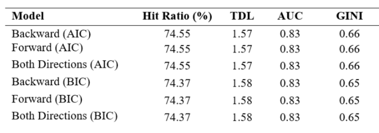
Stepwise Logistic

Instead of manually deciding the variables to include in the model, as was done with the logistic regression method, Stepwise logistic regression is utilized as a feature selection algorithm. The advantage of this method is that it helps identify both important variables and control variables. There are many types of stepwise regression: Forward, Backward, or both. The process involves adding or removing a variable to determine the extent to which it improves the model.

Decisions are based on information criteria, such as the Akaike Information Criterion (AIC) and Bayesian Information Criterion (BIC), along with significance. The process continues until there is no substantial improvement or worsening in the model.

BIC models were chosen, whether using backward, forward, or both directions for model selection. The Akaike Information Criterion tends to favor the complex models, in contrast to the Bayesian Information Criterion, which showed a preference for simpler models (Liu et al., 2023). The variables that were identified through the stepwise regression process are: Income, Relation_length, Start_channel, Email_list, Electricity_usage, Gas_usage, and flexible_contract.

Stepwise Logistic Regression
performance metrics

# Stepwis Logistic Regression ----
## Model estimation ----
Logistic_regression_full <- glm(Churn ~ ., data = estimation_dataset, family = binomial)
Logistic_regression_null <- glm(Churn ~ 0, data = estimation_dataset, family = binomial)
### Backward Stepwise Logistic Regression
Logistic_regression_backward <- stepAIC(Logistic_regression_full, 
                                        direction="backward", trace = TRUE)
### Forward Stepwise Logistic Regression
Logistic_regression_forward <- stepAIC(Logistic_regression_null, direction="forward",
                                       scope=list(lower=Logistic_regression_null, upper=Logistic_regression_full), trace = TRUE)
### Both Directions Stepwise Logistic Regression 
Logistic_regression_both <- stepAIC(Logistic_regression_full, 
                                    direction="both", trace = TRUE)

## Bayesian Informationd Cruterion (BIC) ----
### Backward Stepwise Logistic Regression 
Logistic_regression_backward_BIC <- stepAIC(Logistic_regression_full, direction="backward", 
                                            trace = TRUE, k = log(sum(data$estimation_dataset)))

### Forward Stepwise Logistic Regression 
Logistic_regression_forward_BIC <- stepAIC(Logistic_regression_null, direction="forward", 
                                           scope=list(lower=Logistic_regression_null, upper=Logistic_regression_full), 
                                           trace = TRUE, k = log(sum(data$estimation_dataset)))


### Both Directions Stepwise Logistic Regression
Logistic_regression_both_BIC <- stepAIC(Logistic_regression_full, direction="both", trace = TRUE, 
                                        k = log(sum(data$estimation_dataset)))

## Predictions ----
# AIC Models 
predictions_backward_AIC <- predict(Logistic_regression_backward, type = "response", newdata=validation_dataset)
predictions_forward_AIC <- predict(Logistic_regression_forward, type = "response", newdata=validation_dataset)
predictions_both_AIC <- predict(Logistic_regression_both, type = "response", newdata=validation_dataset)
# BIC Models 
predictions_backward_BIC <- predict(Logistic_regression_backward_BIC, type = "response", newdata=validation_dataset)
predictions_forward_BIC <- predict(Logistic_regression_forward_BIC, type = "response", newdata=validation_dataset)
predictions_both_BIC <- predict(Logistic_regression_both_BIC, type = "response", newdata=validation_dataset)
## Fit Criteria ----
# AIC MODELS
fitcriteria_calculator(predictions_backward_AIC,validation_dataset$Churn)
fitcriteria_calculator(predictions_forward_AIC,validation_dataset$Churn)
fitcriteria_calculator(predictions_both_AIC,validation_dataset$Churn)

#BIC MODELS - Backward, Forward, Both
fitcriteria_calculator(predictions_forward_BIC,validation_dataset$Churn)
fitcriteria_calculator(predictions_backward_BIC,validation_dataset$Churn)
fitcriteria_calculator(predictions_both_BIC,validation_dataset$Churn)

Decision Trees

The Decision Tree Classification model, specifically the CART (Classification and Regression Tree) approach, is another technique explored and evaluated. It comprises a supervised learning method employed to classification tasks. This model operates by partitioning the data in a way that minimizes impurity within each group. It creates nodes by identifying and using the attributes that most significantly reduce impurity until it is minimized. Decision tree models have the capacity to discern and prioritize the most influential attributes within a dataset for a specific task. Initially, the model is trained using the training set, including all the variables and then it is implemented on the testing set to evaluate its performance.

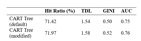
For the aim of this study, two CART models are compared to determine the superior performer. The first model utilizes default parameters, while the second model is adjusted by reducing the complexity parameter from 0.01 to 0.008 and increasing the maximum depth to 4, thus allowing for a more expansive tree. Performance metrics for both models are detailed in Table 4. While the modified model shows slightly improved performance, the default model is preferred due to concerns about overfitting. The adjustments in the second model make the tree excessively specific, potentially reducing its efficiency on a new dataset. Subsequently, the default CART model is preferred.

CART Decision Tree
performance metrics

# CART tree 
# Using the baseline variables
Cart_tree2 <- rpart(Churn ~ Age + Income + Relation_length + Electricity_usage +
                      Gas_usage + flexible_contract + Contract_length + Start_channel +
                      Email_list + Home_label, data=estimation_dataset, method="class")
predictions_cart2 <- predict(Cart_tree2, newdata=validation_dataset, type ="prob")[,2]
rpart.plot(Cart_tree2,extra = 106)

# Changing settings
newsettings1 <- rpart.control(minsplit = 100, minbucket = 50, cp = 0.008, maxdepth = 4)
Cart_tree3 <- rpart(Churn ~ ., data=estimation_dataset, method="class", control=newsettings1)
Cart_tree3_visual <- as.party(Cart_tree3)
# Save predictions
predictions_cart3 <- predict(Cart_tree3, newdata=validation_dataset, type ="prob")[,2]
# Performance Metrics (Remove hashtags to execute them)
# fitcriteria_calculator(predictions_cart2,validation_dataset$Churn)
# fitcriteria_calculator(predictions_cart3,validation_dataset$Churn)

For simplicity, only the selected CART model is showcased.Examining the abobe decision tree, it is revealed that the type of contract, specifically whether it is flexible or not, is the primary determinant of predicting customer churn. This factor comprises the root node of the decision tree. In particular, customers with non-flexible contracts exhibit a 35% likelihood of churning. In contrast, those with fl exible contracts present a 71% propensity to churn.

As the decision tree further branches out, the next most important variable is electricity usage. For customers with fixed contracts and a yearly electricity consumption below 2223 kWh, the churn probability is 22%. Conversely, the tree leads to another split which includes relation length as a splitting rule. In this case, a customer with a relationship greater than 37 months has a probability of almost 40% to defect, while customers with the shortest relationship, present a probability of 58% to terminate their relationship with the company. On the other hand, customers with a flexible contract and electricity usage exceeding 1941 kWh have the greatest probability of defect, at 79%. The last attribute presented in the tree is Gas usage, derived from customers with electricity usage smaller than 1941kWh and indicates that a customer has a 63% probability to churn when gas usage is larger than 979 cubic meters per month.

Overall, the tree model comprehensively identifies which customer segments are more likely to terminate their relationship with the company. In this case, it appears that customers with flexible contracts and high energy consumption are the segments that should be targeted for retention, as they present the greatest probability of churn.

Random Forest

Random Forest is a specific type of ensemble model that builds a collection of decision trees and combines their outputs. It is less prone to overfitting compared to individual decision trees, as the aggregation of multiple trees helps to smooth out individual errors. Random Forest provides a measure of feature importance, indicating which features contribute the most to the model’s predictions.

Two random forests were implemented, one with no settings and the other with 700 trees. However for simplicity, only the results of the best performing are presented. Models score almost the same on the fit criteria, with no settings model scoring slightly better in the Hit Ratio and the Gini Coefficient. The plot below shows that the most important features are the same for both models. More specifically, the top 5 variables, in order of importance, are the Electricity_usage, Gas_usage, Relation_length, Income, and Start_channel.

# Random forest ----
estimation_dataset$estimation_dataset <- NULL
Random_forest1 <- randomForest(Churn ~ ., data=estimation_dataset, importance=TRUE)
predictions_forest1 <- predict(Random_forest1, newdata=validation_dataset, type ="prob")[,2]
# Extract variable importance measures
var_importance <- importance(Random_forest1)

importance_df <- data.frame(Variable = row.names(var_importance), Importance = var_importance[, 1])
# Plot variable importance using ggplot2
ggplot(importance_df, aes(x = Importance, y = reorder(Variable, Importance))) +
  geom_bar(stat = "identity", fill = "lightblue") +
  labs(x = "Importance", y = "Variable") +
  ggtitle("Variable Importance") +
  theme_minimal()

#Fit criteria  Random_forest1
fitcriteria_calculator(predictions_forest1,validation_dataset$Churn)

## HIT RATE INFORMATION: 
##  True Negatives: 1887 
##  False Negatives: 635 
##  True Positives: 1765 
##  False Positives: 598 
##  
##  Hit rate (%):  74.75947 
##  Sensitivity (%):  73.54167 
##  Specificity (%):  75.93561 
##  
##  TOP DECILE LIFT INFORMATION: 
##  TDL value: 1.580119 
##  
##  GINI INFORMATION: 
##  GINI value: 0.6531703 
##  AUC INFORMATION: 
##  AUC value: 0.8265851

Gradient Boosting

Boosting is an ensemble technique that strengthens a model by sequentially integrating many weak learners, the decision trees, to form a robust predictor. It enhances model accuracy by iteratively correcting errors from previous models, with a special focus on data points that are difficult to predict. A Gradient Boosting is applied in our analysis that builds models in succession, each targeting the largest errors until reaching a set accuracy threshold, improving generalization to new data. Boosting works by taking the weighted sum of predictions from all trees, leveraging the greedy nature of decision trees that make splits based on immediate error reduction. By combining the predictions of these trees, Boosting achieves a more accurate and reliable final prediction.

Our model generates 10000 trees, the shrinkage parameter lambda is 0.01 which is the learning rate, and the interaction depth d represents the total number of splits to be performed. So here each tree is a small tree with only 4 splits. The summary of the Model gives a featureimportance plot. The two most important features that explain the maximum variance in the data set are Electricity usage and Contract length. The output shows a hierarchy of model determinants. Electricity usage leads with 22.45%, as the paramount determinant. Contract length (18.80%) and Gas usage (17.32%) follow closely and are also very significant. Age, Home_label, and Home_age have minimal effects (0.43%, 0.39%, 0.11%) and Gender, with no influence at all, excluding it from the model’s key determinators. Partial dependence plots are also implemented to show the relationship between the two most important variables (Electricity usage and Contract length) with the response variable (Churn).

estimation_dataset$estimation_dataset <- NULL
estimation_dataset$Churn <- as.integer(as.character(estimation_dataset$Churn))
# Model Estimation
boost_tree1 <- gbm(Churn ~ ., data=estimation_dataset, 
                   distribution = "bernoulli", n.trees = 10000, 
                   shrinkage = 0.01, interaction.depth = 4)
# Print the results
boost_tree1

## gbm(formula = Churn ~ ., distribution = "bernoulli", data = estimation_dataset, 
##     n.trees = 10000, interaction.depth = 4, shrinkage = 0.01)
## A gradient boosted model with bernoulli loss function.
## 10000 iterations were performed.
## There were 13 predictors of which 13 had non-zero influence.

# Best Iteration 
best.iter <- gbm.perf(boost_tree1, method = "OOB",plot.it = FALSE)

## OOB generally underestimates the optimal number of iterations although predictive performance is reasonably competitive. Using cv_folds>1 when calling gbm usually results in improved predictive performance.

summary(boost_tree1, n.trees = best.iter, plotit = FALSE)

##                                 var     rel.inf
## Electricity_usage Electricity_usage 22.60552485
## Contract_length     Contract_length 18.67055470
## Gas_usage                 Gas_usage 17.25495653
## flexible_contract flexible_contract 13.63781098
## Relation_length     Relation_length 10.15601191
## Income                       Income  8.09541464
## Start_channel         Start_channel  3.75764901
## Email_list               Email_list  2.96957237
## Province                   Province  1.84298000
## Age                             Age  0.47635397
## Home_label               Home_label  0.39945627
## Home_age                   Home_age  0.12891768
## Gender                       Gender  0.00479708

# Boosting predictions
predictions_boost1 <- predict(boost_tree1, newdata=validation_dataset, n.trees = best.iter, type ="response")
# Fit criteria
fitcriteria_calculator(predictions_boost1,validation_dataset$Churn)

## HIT RATE INFORMATION: 
##  True Negatives: 1924 
##  False Negatives: 598 
##  True Positives: 1770 
##  False Positives: 593 
##  
##  Hit rate (%):  75.61924 
##  Sensitivity (%):  74.74662 
##  Specificity (%):  76.44021 
##  
##  TOP DECILE LIFT INFORMATION: 
##  TDL value: 1.6013 
##  
##  GINI INFORMATION: 
##  GINI value: 0.6779132 
##  AUC INFORMATION: 
##  AUC value: 0.8389566

Support Vector Machine

Support Vector Machines is a supervised machine learning algorithm used for classification. It operates by constructing a hyperplane in a feature space that distinctly separates instances belonging to different classes. The goal is to find the hyperplane with the maximum margin, which is the distance between the hyperplane and the nearest data points from each class.

These nearest data points are referred to as support vectors. The optimization process in SVM involves minimizing the classification error while maximizing the margin, making it a robust algorithm for both linear and non-linear classification tasks. Additionally, SVM can handle high-dimensional data efficiently. Four different kernel functions were conducted: Linear Kernerl, Polynomial Kernel, Sigmoid Kernel, and Gaussian Radial Basis Function (RBF) (For simplicity reasons only the best performing is presented). The variables that were used are the ones that were used for the baseline model. Fit criteria identified the Gaussian Radial Basis Function (RBF) as the optimal model among the four, outperforming all others across all criteria (Table 9). The only substantial plot is depicted in Figure 9, illustrating the relationship between age and electricity usage. In particular, the classification of people as churners increases when their age increases and electricity consumption is above 3000, but after their 60th year, the classification of churners decreases as they get older.

## Gaussian Radial Basis Function (RBF) ----- 
svm_3 <- svm(Churn ~ Gender + Age + Income + Relation_length + Contract_length + Electricity_usage + Gas_usage + flexible_contract, data = data, importance=TRUE,
             type = 'C-classification', probability = TRUE,
             kernel = 'radial')

plot(svm_3, data, Electricity_usage~Age) 

# Get predictions
predictions_svm3 <- predict(svm_3, newdata=validation_dataset, probability=TRUE)
predictions_svm3 <- attr(predictions_svm3,"probabilities")[,1]
# Fit criteria for Gaussian Radial Basis Function (RBF)
fitcriteria_calculator(predictions_svm3,validation_dataset$Churn)

## HIT RATE INFORMATION: 
##  True Negatives: 1930 
##  False Negatives: 592 
##  True Positives: 1733 
##  False Positives: 630 
##  
##  Hit rate (%):  74.98465 
##  Sensitivity (%):  74.53763 
##  Specificity (%):  75.39062 
##  
##  TOP DECILE LIFT INFORMATION: 
##  TDL value: 1.622482 
##  
##  GINI INFORMATION: 
##  GINI value: 0.6467897 
##  AUC INFORMATION: 
##  AUC value: 0.8233948

Managerial Conclusion

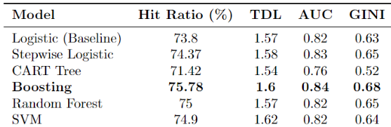
It is determined from the models that the variables that have the most substantial influence on churning are service usage (electricity & gas usage), contract length, flexible contract, and relation length. Gradient boosting is chosen as the best model for the Dutch Energy Supplier, based on the performance metrics. The performance metrics suggest that the Boosting model exhibits the highest predictive capability, representing a significant enhancement over the baseline model. More specifically, it has the highest scores in fit criteria with a Hit Ratio of 75.78%, TDL of 1.6, AUC of 0.84, and Gini Coefficient of 0.68.

After the execution of Partial Dependence Plots, where the relation and direction between important variables and target variable are revealed, it is concluded that service usage influence positively on churn. In other words, as the service usage increases, the probability of churn increases. Consequently, the hypothesis that service usage potentially leads to lower churn rates is rejected in our study. Regarding the contract length it is found that customers possessing extended contract terms demonstrated diminished churn rates, aligning with the hypothesis outlined in the literature review. As for the hypothesis on relationship length positing a negative impact on the probability of churn, the results confirm the anticipated negative relationship.

Performance metrics for all models

Thus, in order to enhance customer retention, the Dutch energy supplier is recommended to develop and promote energy-efficiency programs for customers with higher usage, which can lead to cost savings and increased customer satisfaction. Furthermore, it is advisable to establish loyalty programs that reward long-term customers, such as offering discounts or exclusive services to those with extended contract terms. This will help in strengthening the company’s relationship with the customers. Lastly, more attention has to be given to the creation of blog posts and educational videos to help the customers understand the long-term benefits and potential savings of staying with the company.

Appendix

1. R libraries needed

To successfully execute this project, the following R libraries are required:

# Loading necessary libraries
library(tidyr)
library(corrplot)
library(ggplot2)
library(dplyr)
library(ROCR)
library(randomForest)
library(reshape2)
library(e1071)
library(rpart)
library(rpart.plot)
library(partykit)
library(MASS)
library(gbm)
library(neuralnet)

2. Detailed dataset description

1. Customer_ID: a unique customer identification number.
   
2. Gender: a dummy variable indicating if the customer who signed the contract is male (0) or female (1).
   
3. Age: the age of the customer in years.
   
4. Income: the monthly income of the customer’s household in euros.
   
5. Relation_length: the amount of months the customer has been with the firm.
   
6. Contract_length: the amount of months the customer still has a contract with the firm. Zero
   means the customer has a flexible contract, i.e., (s)he can leave anytime without paying a
   fine. If the contract is more than zero months, the customer can still leave, but has to pay a
   fine when leaving.
   
7. Start_channel: indicating if the contract was filled out by the customer on the firm’s website (“Online”) or by calling up the firm (“Phone”).
   
8. Email_list: indicating if the customer’s email address is known by the firm (1=yes, 0=no).
9. Home_age: the age of the home of the customer in years.
   
10. Home_label: energy label of the home of the customer, ranging from A (good) to G (bad).
11. Electricity_usage: the yearly electricity usage in kWh.
    
12. Gas_usage: the yearly gas usage in cubic meters.
    
13. Province: the province where the customer is living.
    
14. Churn: a dummy variable indicating if the customer has churned (1) or not (0)
    

3. Fit Criteria Custom Function

The fitcriteria_calculator function assesses binary classification model performance. It calculates hit rate, sensitivity, specificity, top decile lift (TDL), and plots a lift curve. Additionally, it computes the Gini coefficient and the area under the ROC curve (AUC), providing a comprehensive evaluation of the model’s predictive accuracy and discriminative capacity * Execute this custom function in the beggining of the script.

# Custom function calculator for fit criteria 
fitcriteria_calculator <- function(predict, IV) {
  tablebase <- ifelse(predict > .5, 1, 0)
  
  # HIT RATE CALCULATIONS
  hitrate_table <- table(IV, tablebase, dnn = c("Observed", "Predicted"))
  hit_rate <- ((hitrate_table[1,1] + hitrate_table[2,2]) / sum(hitrate_table)) * 100
  sensitivity <- (hitrate_table[2,2] / (hitrate_table[2,2] + hitrate_table[1,2])) * 100
  specificity <- (hitrate_table[1,1] / (hitrate_table[1,1] + hitrate_table[2,1])) * 100
  
  # TDL CALCULATIONS (10 levels)
  decile_ntile <- ntile(tablebase, 10)
  decile_table <- table(IV, decile_ntile, dnn = c("Observed", "Decile"))
  tdl <- (decile_table[2,10] / (decile_table[1,10] + decile_table[2,10])) / mean(IV)
  
  # LIFT CURVE PLOT
  pred <- prediction(predict, IV)
  perf <- performance(pred, "tpr", "fpr")
  plot(perf, xlab = "Cumulative % of observations", ylab = "Cumulative % of positive cases", xlim = c(0, 1), ylim = c(0, 1), xaxs = "i", yaxs = "i", main = "Lift Curve") + abline(0, 1, col = "red")
  
  # GINI AND AUC CALCULATIONS
  auc_perf <- performance(pred, "auc")
  auc <- as.numeric(auc_perf@y.values)
  gini <- auc * 2 - 1
  
  # Output
  cat('HIT RATE INFORMATION:', '\n', 'True Negatives:', hitrate_table[1,1], '\n', 'False Negatives:', hitrate_table[1,2], '\n', 'True Positives:', hitrate_table[2,2], '\n', 'False Positives:', hitrate_table[2,1], '\n',
      '\n', 'Hit rate (%): ', hit_rate, '\n', 'Sensitivity (%): ', sensitivity, '\n', 'Specificity (%): ', specificity, '\n', '\n',
      'TOP DECILE LIFT INFORMATION:', '\n', 'TDL value:', tdl, '\n', '\n',
      'GINI INFORMATION:', '\n', 'GINI value:', gini, '\n',
      'AUC INFORMATION:', '\n', 'AUC value:', auc)
}

Note that the `echo = FALSE` parameter was added to the code chunk to prevent printing of the R code that generated the plot.